Why Z-Score Fails — and %-Change Lets a PPO Agent Trade

When working with reinforcement learning on financial time series, one of the most overlooked yet critical steps is how you preprocess your data — especially normalization. In this article, we take a step back from complex architectures and real-world noise to focus on the fundamentals: Can a simple PPO agent learn a predictable, profitable pattern from just a single close-price time series?

To answer that, we generate a synthetic dataset with clear, repeatable patterns and use a straightforward MLP model — no LSTMs, no Transformers. Our goal is to establish a reliable testing ground that proves: yes, learning is possible, but only if the data is properly prepared.

This hands-on experiment isn't about theory — it's about making reinforcement learning work in practice. While many academic papers and thesis projects offer elegant math and complex setups, they often fail to answer a simple question: what does it take to make a basic model learn something meaningful?

We'll show how normalization — both via z-score and percent-change — directly affects whether the model learns at all. This post is for anyone who's tired of abstract discussions and wants to see concrete results, with code and data that actually do the job.

Chapter 1: Creating the Synthetic Dataset

To train a reinforcement learning agent effectively, we need a dataset that allows the model to learn. This sounds trivial, but in practice, most real-world financial data is noisy, chaotic, and often lacks clear, repeatable signals — especially when starting with a minimal setup like a single "close" price time series.

In this first step, we generate a fully synthetic time series that simulates a year of hourly close prices.

"""Generate synthetic financial close price data with repeatable patterns
for training reinforcement learning models."""

import random
import matplotlib.pyplot as plt
import pandas as pd
import numpy as np

# Setup: define time range and initialize close price array
NUM_HOURS = 8064
start_time = pd.Timestamp("2024-01-01 00:00:00")
time_index = pd.date_range(start=start_time, periods=NUM_HOURS, freq="h")
close = np.zeros(NUM_HOURS)

# Set starting close price
close[0] = 100.0

# Create random number generator (for reproducibility)
rng = np.random.default_rng(seed=42)

# Inject daily repeatable pattern every day at 10:00
pattern_indices = []
for day in range(NUM_HOURS // 24):
    base = day * 24 + 10
    if base + 5 < NUM_HOURS:
        pattern_indices.append(base)

# Generate close prices with random variation and inserted patterns
i = 1
while i < NUM_HOURS:
    if i in pattern_indices:
        # Create upward trend for 5 hours (+0.3% per hour)
        for j in range(5):
            if i >= NUM_HOURS:
                break
            close[i] = close[i - 1] * 1.003
            i += 1
        # Sharp drop of -1.5% after the upward pattern
        if i < NUM_HOURS:
            close[i] = close[i - 1] * 0.985
            i += 1
    else:
        # Otherwise apply random walk with small variation
        delta = random.uniform(-0.002, 0.002)
        close[i] = close[i - 1] * (1 + delta)
        i += 1

# Save to CSV for further processing
df = pd.DataFrame(data={"close": close}, index=time_index)
df.to_csv("synthetic_close_data.csv")

# Plot the synthetic close prices
plt.figure(figsize=(12, 4))
plt.plot(close, label="Close Price", linewidth=1)
plt.title("Synthetic Close Price Time Series")
plt.xlabel("Time Step (hour)")
plt.ylabel("Close Price")
plt.grid(True, linestyle="--", alpha=0.5)
plt.legend()
plt.tight_layout()
plt.show()

The core idea behind the code is simple: we inject a repeatable, tradable pattern every 24 hours. Specifically, at the same time each day (10:00), the synthetic price begins a 5-hour upward trend (+0.3% per hour), followed by a sharp drop of -1.5%. The rest of the time, the price behaves like a random walk with slight fluctuations (±0.2%).

This deterministic pattern is intentionally easy to exploit — if the model can't learn this, it certainly won't learn more subtle patterns in real financial markets. The simplicity allows us to focus on core mechanics like data normalization, reward shaping, and model behavior without being distracted by market noise.

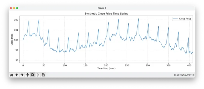
The result is a clean training environment where we can observe whether the agent detects and acts upon the embedded opportunity. In the chart above, you can clearly see the repeated price ramps and drops — the signature our model should learn to trade. This visual confirmation gives us a solid baseline before we move on to more complex scenarios.

Chapter 2: We Need a Training Environment

Before we dive into real-world data or advanced strategies, we need one thing first: a stable and understandable training environment. In this project, the focus is not on building complex Gym wrappers or experimenting with exotic model architectures — we focus on the data and the reward function, because that's what really drives learning in reinforcement learning (RL) setups.

There are countless tutorials on how to set up a PPO environment using OpenAI Gym or Gymnasium. If you're reading this, chances are you've already seen some of them. So we'll keep it simple and skip the boilerplate.

We use Stable Baselines3 (SB3) because it's reliable, readable, and beginner-friendly. Sure, it's not perfect — scaling beyond a single machine is limited, and you'll hit walls eventually if you want distributed training. But for experimentation, debugging, and fast iteration, it's hard to beat. Rewriting everything in raw PyTorch, using RLlib or PyTorchRL, is massive overkill at this stage. You don't want to debug your framework before you debug your idea.

To improve the training quality, we use Maskable PPO, a variant of PPO that supports action masking. This means the model learns faster and more efficiently by being told in each step which actions are even valid. In our case, the action space is very simple — 4 discrete actions:

• 0: open a short position
• 1: hold
• 2: open a long position
• 3: close an open position

def _get_action_mask(self):
    mask = np.array([0, 1, 0, 0], dtype=np.int8)
    if self.position == 0:
        mask[0] = 1  # short
        mask[2] = 1  # long
    else:
        mask[3] = 1  # close
    return mask

Only some of these actions are allowed depending on the current position — e.g., you can't "close" if there's no trade open. Action masking helps the model avoid wasting learning capacity on invalid actions, and this has a huge impact on learning speed and stability.

The agent is trained using a small and simple MLP: two layers with 128 and 64 units. But — and this is crucial — we don't feed it raw flat input. We use a 1D Convolutional Neural Network (CNN) to extract features from the time series window. This gives us temporal pattern recognition without needing an LSTM or Transformer. We also include a small feedforward network for context input — specifically, the current position (long, short, or flat). The combined output is then passed into the MLP for action prediction.

This hybrid approach gives us the power of sequence modeling (via CNN) and context awareness (via a tiny context net), without the overhead or complexity of recurrent or attention-based architectures. It's fast, clean, and absolutely sufficient to prove that a pattern can be learned.

model = MaskablePPO(
    policy=TradingPolicy,
    env=train_env,
    gamma=0.98,
    clip_range=0.1,
    n_epochs=10,
    batch_size=64,
    normalize_advantage=True,
    learning_rate=1e-4,
    tensorboard_log="tensorboard_exam/",
    policy_kwargs=dict(
        activation_fn=torch.nn.ReLU,
        net_arch=[128, 64],
        context_input_dim=1,
        cnn_out_channels=64,
        cnn_kernel_size=5,
    ),
    verbose=1
)

In addition to defining the policy_kwargs when instantiating the model, it's important to note that both the feature extractor and the custom trading policy must be implemented manually. If you're interested in the full training setup or want to see the exact environment implementation, feel free to reach out — I'm happy to share more details. I've intentionally left out the boilerplate here to keep the focus on what's essential.

In short: we're not trying to build the perfect pipeline. We're trying to build something that works — and that lets us isolate the real questions: Did the model learn something useful? Did normalization help? That's what comes next.

Chapter 3: The Reward Function

If reinforcement learning is about learning through experience, then the reward function is the teacher. It tells the agent whether its actions were good, bad, or irrelevant — and in doing so, it shapes everything the model learns.

In our setup, the reward function is intentionally simple, but incredibly effective for the task at hand. It's embedded inside the step() method of our custom trading environment, and it governs how the agent is rewarded or penalized for taking actions like going long, going short, holding, or closing a position.

def step(self, act):
    price = self.price[self.ptr]
    reward = 0.0

    if act == 2:  # long
        if self.position == 0:
            self.position = 1
            self.entry_price = price
    elif act == 0:  # short
        if self.position == 0:
            self.position = -1
            self.entry_price = price
    elif act == 3:  # close
        if self.position != 0:
            if self.position == 1:
                pnl = (price - self.entry_price) / self.entry_price
            else:  # short
                pnl = (self.entry_price - price) / self.entry_price
            reward = pnl
            self.position = 0
            self.entry_price = 0.0
    elif act == 1:  # hold
        if self.position != 0:
            pnl = (price - self.entry_price) / self.entry_price * self.position
            reward += pnl * 0.01

    self.ptr += 1
    done = self.ptr >= len(self.price) - 1

    if done and self.position != 0:
        if self.position == 1:
            pnl = (price - self.entry_price) / self.entry_price
        else:
            pnl = (self.entry_price - price) / self.entry_price
        reward += pnl
        self.position = 0
        self.entry_price = 0.0

    info = {"action": act, "reward": reward}
    return self._obs(), reward, done, False, info

Here's what it does, in essence:

• If the agent opens a long or short trade, it receives no immediate reward — the trade has just begun.
• If the agent closes a position, it receives the full profit or loss (PnL) of that trade, calculated as the percentage change in price since the entry.
• If the agent holds an open position, it receives a small scaled reward based on the unrealized PnL. This encourages it to let profitable trades run — but only when it makes sense.
• If the episode ends and a trade is still open, the environment forces a close, and the final PnL is rewarded.

This structure is simple but captures the essence of trading: the agent is encouraged to enter good positions and close them at the right time, while avoiding trades that lead to losses. The reward is sparse — but not too sparse. It's shaped just enough to help the model learn when to act and when to wait.

What makes this work is the synthetic data we designed earlier. The reward function is able to clearly reflect whether the model has learned to recognize the daily pattern we injected. If it does, we expect the following behavior:

1. The agent opens a long position right at the beginning of the pattern (around 10:00).
2. It holds during the upward price movement.
3. It closes before the sharp drop and opens a short position.
4. It holds until the bottom is reached, then closes the trade.
5. Everything else — in the best case, nothing. Just waiting for the next spike.

By designing a transparent reward function that aligns directly with the structure of the data, we remove a major source of uncertainty in RL training. Once this works, we can increase complexity — but only once we've proven that the fundamentals are solid.

Chapter 4 (Act I): Z-Score Normalization

We'll start our normalization journey with the classic: z-score normalization. It's simple, widely used, and — crucially — removes absolute price level effects so the model can focus on relative structure in the data.

# Z-Score Normalization
close = df_raw["close"]
close_norm = (close - close.mean()) / close.std()
df = pd.DataFrame({"close": close_norm}, index=close.index)

What it does

Z-score normalization centers the series at mean = 0 and rescales it so the standard deviation = 1 (approximately, up to floating error). That means:

• Price levels (e.g., 100 vs. 150 vs. 80) no longer matter.
• The daily synthetic spike pattern we injected earlier now shows up as structured positive deviations, followed by negative reversals, all in standardized units ("how many sigmas away from average").
• Background noise collapses into a tighter band around zero, making the spike pattern stand out more cleanly.

Tip: In production you normally compute mean/std on the training split only to avoid look-ahead bias. Here — in a fully synthetic, didactic setting — we normalize across the full dataset for clarity. We'll still evaluate on unseen splits to check generalization.

What the dataset looks like afterward

Instead of a drifting price curve, you now see a standardized oscillating series: long stretches near 0 with recurring multi-sigma moves where our +0.3% × 5-up / −1.5% drop pattern kicks in. These recurring excursions are exactly what we want the PPO agent to detect and trade. The normalization removes the distraction of absolute price scale so training can focus on shape.

Train/Val/Test splits to limit bias

We split the time series chronologically (e.g., 60% train / 20% validation / 20% test). The daily spike structure remains, but the levels and random walk noise between spikes differ in the validation and test portions. That matters: the model can't just memorize absolute values; it must respond to standardized moves.

We train the Maskable PPO agent for 500k steps on the z-score–normalized data.

The result: meh, not exactly great

1. Cumulative Reward: The Collapse

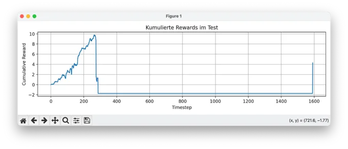
At first glance, the training seemed to work: we see an early accumulation of rewards. But then, around timestep 300, everything falls apart. The model takes a series of bad trades and crashes into a negative reward zone, from which it never recovers. The agent continues through the episode without ever recovering, and barely trades at all. That's a sign that it completely lost signal — and confidence.

2. Test Overview: A Confused Start, Then Silence

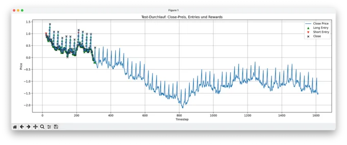
Looking at the full test run, we see the agent trying both long and short positions early on. But its behavior is chaotic — entries seem random, closes are frequent but erratic. Once the price drifts far enough from the original z-score distribution (i.e. shifts too far in standardized terms), the agent completely stops trading. No action appears valid or rewarding anymore.

3. Zoom Detail: Nothing but Holds

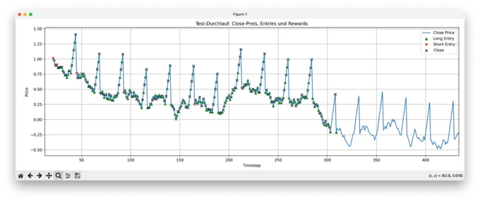
Zooming in reveals what's happening: random long positions and after a certain point, the agent only executes hold actions. No entries, no closes — just passivity. This is a classic failure mode of PPO in poorly shaped environments: if the model can't connect its actions to positive rewards, it defaults to "do nothing" as the safest option.

Chapter 4 (Act II): % Normalization

In this part, we switch from z-score normalization of raw close prices to something more aligned with how financial time series behave: percent change normalization.

Instead of feeding absolute prices into the model (even normalized ones), we now work with percentage returns — the relative change from one timestep to the next. These percent changes are then themselves normalized (again via z-score) to ensure a consistent scale for learning:

# Percent-change + normalization for training, keep raw close for PnL
close = df_raw["close"]
pct_change = close.pct_change().fillna(0)
pct_norm = (pct_change - pct_change.mean()) / pct_change.std()
df = pd.DataFrame({
    "close": close,
    "feature": pct_norm
}, index=close.index)

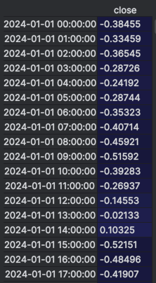
The screenshot below shows a raw excerpt from the dataset after applying percent-change normalization. The close column contains the original price, while the feature column shows the normalized percentage change used as input for training.

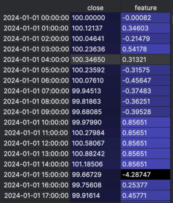
Even without any plotting, you can already see the daily pattern forming — look at the sequence starting from 2024-01-01 10:00:00 to 14:00:00. The feature values jump to 0.85651 consistently for several hours, which corresponds to our synthetic +0.3% per hour increase. Then, at 15:00:00, the sharp drop is reflected as a highly negative normalized value: -4.28747. That's our -1.5% cliff.

This table alone shows why percent-change normalization is so effective: the repeating spike pattern stands out clearly in the normalized feature column. It makes the job for the model (and for us) much easier — it no longer has to "guess" whether a move is big or small. Everything is standardized, and patterns become explicit.

Why this matters

With percent normalization, we're telling the model: "Don't learn based on price levels — learn based on how fast and in which direction things are moving."

This is a crucial mindset shift, and one that mirrors how most real-world trading models work. Markets behave in relative terms. A +1% move on a $10 stock is just as relevant as on a $1,000 stock. Price level ≠ signal.

Visual clarity

You'll notice it immediately when plotting the normalized data: the spike pattern becomes visually obvious. No more masking by price drift or trend. You can see the five consecutive +0.3% moves, and the following -1.5% drop, now standardized and clean. The recurring wave is no longer buried in scale — it's front and center. Compared to the z-score normalized close prices, which still carry embedded structure from absolute levels, this version reveals the pattern much more clearly. The model benefits from that too.

Training with this representation

Just like before, we train our agent with 500,000 steps. The key difference is:

• We still retain the original close values in the dataframe.
• But these are not used during training — only for computing profit and loss (PnL) when trades are opened and closed.

This setup reflects a clean separation of observation (what the agent sees) vs. outcome (what defines reward). The model trains on normalized percent changes, but reward is always calculated in real money terms using actual price differences.

The result: it works

1. Full Test Set: Model Actions

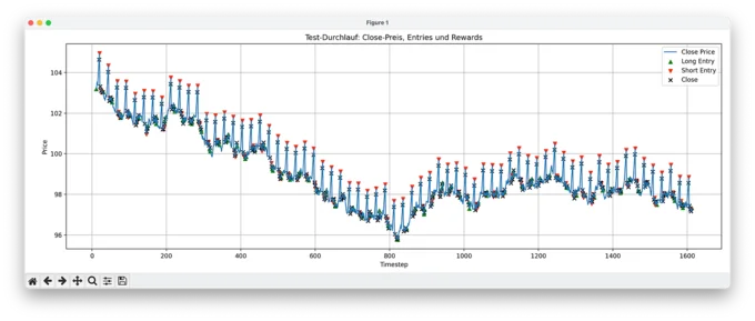
In this plot, we see the model's predicted actions over the full test set. Despite the drifting and volatile price levels, the model opens trades precisely at the right moments: entering long before upward spikes, short before downturns, and consistently closing positions in time. The fact that it performs this well without access to price level information confirms that the normalization worked and the pattern was learned.

2. Zoomed-In View: Action Detail

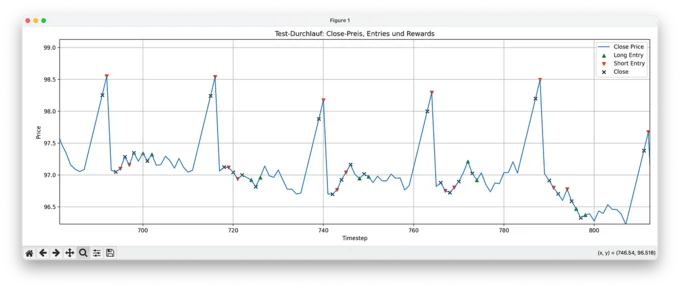
Zooming in, we can observe individual long and short entries with their corresponding closes. The behavior isn't perfectly deterministic (nor should it be with PPO), but it's consistent and robust. The model has clearly learned to anticipate the repeating spike pattern and makes mostly profitable decisions.

3. Cumulative Reward Over Time

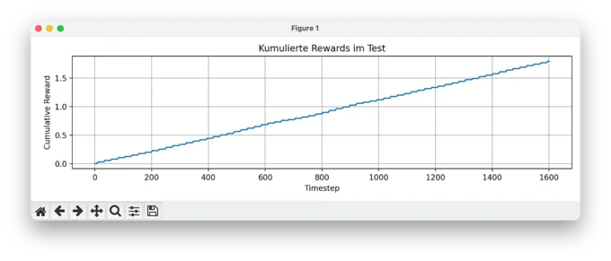
Lastly, the cumulative reward plot shows exactly what we hoped for: a smooth, stable increase without drawdowns. No sudden losses, no reward volatility — just a clean reward curve that confirms the model is making good trades, over and over.

Conclusion

In summary, switching to percent-change normalization helped the model focus on what matters. By stripping away irrelevant price scale and training on consistent patterns of return behavior, we enabled even a simple MLP+CNN agent to learn highly effective trade timing with just a close price — demonstrated through strong performance and visual clarity in test results.