In the search for understandable and practical guides on how to train a Long Short-Term Memory (LSTM) model with Reinforcement Learning (RL) using PyTorch, one often encounters numerous theoretical and scientifically complex documentations. Unfortunately, there are only a few practical examples that allow for hands-on learning about how such a model actually works and what the impact of various hyperparameters is, without having to study the field in depth.
This project was born out of the need to create a simple and functional foundation that serves as an entry point into the world of RL and LSTM when simpler models are no longer sufficient. It is aimed at developers, data scientists, and AI enthusiasts who already have basic knowledge in Python and machine learning but are new to the concepts of Reinforcement Learning and recurrent neural networks.
Our goal is to demonstrate how to train an LSTM model with RL to better understand the concepts and their implementation. For this purpose, we have devised a very, very simple problem that has no practical use in reality. However, it is so simple that one can easily understand and, most importantly, control the logic behind the reward system.
This article provides a practical and easy-to-understand guide that enables you to conduct your own experiments and explore the capabilities of these technologies.
The complete project with the source code can be found on GitHub: simple_RL-LSTM. Please refer to this alongside reading the article to observe the behavior of the entire system. We intentionally refrain from explaining the entire code here, as it should be sufficiently documented inline.
The Problem
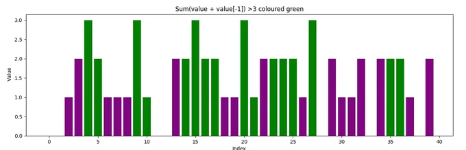
The problem we want to solve is to recognize a specific pattern in a series of data points. For this, we create an array of 1000 tuples with randomly generated values between 0 and 1.
data = np.array(
    [[random.randint(0, 1), random.randint(0, 1), random.randint(0, 1)]
     for i in range(1000)]
)
We are looking for all tuples in this array where the sum of the tuple and the preceding tuple is greater than 3. In the plot, these are represented by all the green bars.
The goal is to teach an LSTM through RL to recognize these sequences on its own. For this, we use the principle of reward and punishment: each time the training process selects the "correct" action for the current tuple, we reward it. In all other cases, we simply do not, thus the LSTM should learn to recognize the logic defined in the step function. The step function is called individually for each bar (each tuple) during training, calculates the reward, and determines the next step.
def step(self, action):
    """
    Takes a step in the environment based on the given action.

    Args:
        action (int): The action to be taken.

    Returns:
        tuple: A tuple containing the next state (torch.Tensor),
        the reward (torch.Tensor), and a boolean indicating if the
        episode is done.
    """
    reward = torch.tensor(0.0, device=self.device)  # No reward in general
    if action == 0 and (torch.sum(self.state[-1]) + torch.sum(self.data[self.current_step - 1]) > 3):
        reward = torch.tensor(10.0, device=self.device)  # Higher reward when the sum is greater than 3

    self.current_step += 1
    if self.current_step >= len(self.data):
        done = True
        self.state = torch.zeros_like(self.state)  # Dummy state when done
    else:
        self.state = self.get_state()
        done = False

    return self.state, reward, done
We see here that only when the action is "0" and the sum of the current tuple (or bar) and the preceding tuple is greater than 3, we reward the selection of action "0" with 10 points.
In this example, the model can choose between three actions from "0" to "2". When choosing "1" or "2", nothing happens. In theory, we could define any number of actions, but this would affect the model and its performance. For our purposes here, three possible actions are sufficient for experimentation.
The Forward Function
It is very important to understand the forward function of the model. This function provides us with the next action to choose based on the current data.
def forward(self, x, hidden):
    """
    Defines the forward pass of the model.

    Args:
        x (torch.Tensor): The input tensor of shape
            (batch_size, sequence_length, input_size).
        hidden (tuple): A tuple containing the initial hidden state
            and cell state of the LSTM.

    Returns:
        torch.Tensor: The output tensor of shape (batch_size, output_size).
        tuple: The hidden state and cell state of the LSTM.
    """
    out, hidden = self.lstm(x, hidden)
    out = self.fc(out[:, -1, :])  # Use the output of the last LSTM cell
    return out, hidden
For x, you need to imagine that we always provide the LSTM with three tuples (or bars): the current one and the two preceding ones. For more complex sequences to find in longer time frames you have to increase the amount of historic data you pass here. Here we just need at least two tuples because we just search for a sequence within the last tuple, I decided to take three to see that it works too. For example:
x = [
    [0, 0, 0],
    [1, 0, 0],
    [1, 1, 1]  # The current bar
]
Together with the reward calculated in the previously mentioned step function, the LSTM learns that when it sees this pattern, it receives a reward if it selects action "0" because the current tuple has a sum of 3 and the preceding one has a sum of 1. Together, this makes 4, and thus we reward action "0", as defined in the step function.
The Training Loop
The actual "learning" takes place in the train function of the agent.
next_q_values, _ = self.model(next_state.unsqueeze(0), next_hidden)
# Add batch dimension with 'unsqueeze(0)'!

q_value = q_values[0, action]
next_q_value = reward + self.gamma * next_q_values.max(1)[0] * (1 - done)

loss = self.loss_fn(
    q_value.unsqueeze(0).unsqueeze(0),
    next_q_value.unsqueeze(0)
)

self.optimizer.zero_grad()
loss.backward()
self.optimizer.step()
Here, we calculate the "loss" which indicates how far the result (i.e., the chosen action in consideration of the current tuples) is from the expected result. This is where the reward comes into play, pushing our result into the positive if the correct action was chosen. The expected result, remember we are dealing with RL, is determined by the model itself!
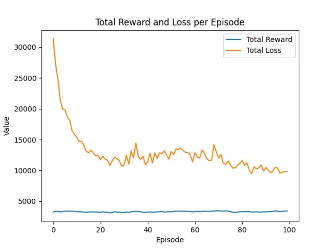
If we look at the results, your loss values should decrease over time, and the received rewards should stabilize along with the loss. The more rewards, the better.
Reading the Output
If you check out the GitHub code and run it (check the README.md for instructions), you should see the following on the console:
Using only the CPU for demonstration purposes
The sum of a datapoint and the previous point which are greater than 3, 350 times.
Episode 10/100,  Total Reward: 3350.0, Total Loss: 15853.9267578125, Action counts: {0: 943, 1:  41, 2: 16}
Episode 20/100,  Total Reward: 3240.0, Total Loss: 12382.6552734375, Action counts: {0: 891, 1: 102, 2:  7}
Episode 30/100,  Total Reward: 3170.0, Total Loss: 10662.9511718750, Action counts: {0: 849, 1: 143, 2:  8}
Episode 40/100,  Total Reward: 3170.0, Total Loss: 10973.5380859375, Action counts: {0: 864, 1: 135, 2:  1}
Episode 50/100,  Total Reward: 3290.0, Total Loss: 11847.7187500000, Action counts: {0: 889, 1:  96, 2: 15}
Episode 60/100,  Total Reward: 3280.0, Total Loss: 11381.9814453125, Action counts: {0: 886, 1: 107, 2:  7}
Episode 70/100,  Total Reward: 3440.0, Total Loss: 13044.0615234375, Action counts: {0: 933, 1:  18, 2: 49}
Episode 80/100,  Total Reward: 3280.0, Total Loss: 11142.7060546875, Action counts: {0: 921, 1:   2, 2: 77}
Episode 90/100,  Total Reward: 3280.0, Total Loss:  9902.1806640625, Action counts: {0: 929, 1:   1, 2: 70}
Episode 100/100, Total Reward: 3400.0, Total Loss:  9808.3828125000, Action counts: {0: 953, 1:  17, 2: 30}
Using only the CPU for demonstration purposes
Percentage: 100.00%, Number of sums > 3: 3680, Total sum of rewards: 3680.0
We see here that with each episode run on the same data, a consistently good reward is achieved. This is because our problem is very simple, and the LSTM quickly understands what it is about. However, pay attention to the fluctuations and try to understand that it is correct that we do not always receive all possible rewards — the model is meant to learn. This is partly determined by the epsilon-greedy factor in the agent, which ensures that our model always experiments a bit with the responses to achieve new results. Another topic not important yet.
We also see that the loss constantly decreases and the number of chosen actions focuses on action "0". It will be interesting later in your real application when multiple actions are dynamically rewarded.
Since we also implemented a test() function in the run.py script, we see the result of our work in the last line. It is important to regularly monitor the success of the training; our test function can be called at any time. It generates a new, random array of tuples and lets the just-trained model select an action for each tuple. If the action was "0" for tuples where the sum with the preceding tuple is greater than 3, we count the response as correct. In this example, the model safely recognized all these 3680 tuples.
Initializing the LSTM
Before you get started, it's important to mention how we initialize the LSTM.
agent = TripleActionAgent(
    input_size=3,
    hidden_size=6,
    output_size=3,
    device=device,
    learning_rate=0.001
)
We use a value of 3 for the input_size, which should always be the number of features you provide to the model. In our case, we use a tuple with three integers of either 0 or 1. Imagine you are calculating a climate model for your region; one feature could be the measured temperature, another the time of day, and the third the humidity.
The hidden_size determines the number of neurons in our hidden layer. We only have one hidden layer here, but you can and often should use more under different circumstances. Hopefully, you will be able to assess this yourself over time. In our case, we use the number of features multiplied by 2.
Simpler is the size of the output_size, which indicates how many possible actions we get at the end. So "0", "1", or "2" in our case which totals three.
Very important is to play around with the learning_rate, we start with 0.001 in this example. The larger this value, the more adjustments will be made to the neural network per iteration. This can lead to significant jumps in learning success and cause your reward values and loss function to fluctuate unpredictably, preventing your model from learning effectively. Small changes in the right direction lead to success.
Now It's Your Turn
Now it's your turn. Load your data, think about how you can calculate the reward for your problem in the step function, and be prepared for the fact that nothing will work perfectly right away.